Running a basic simulation

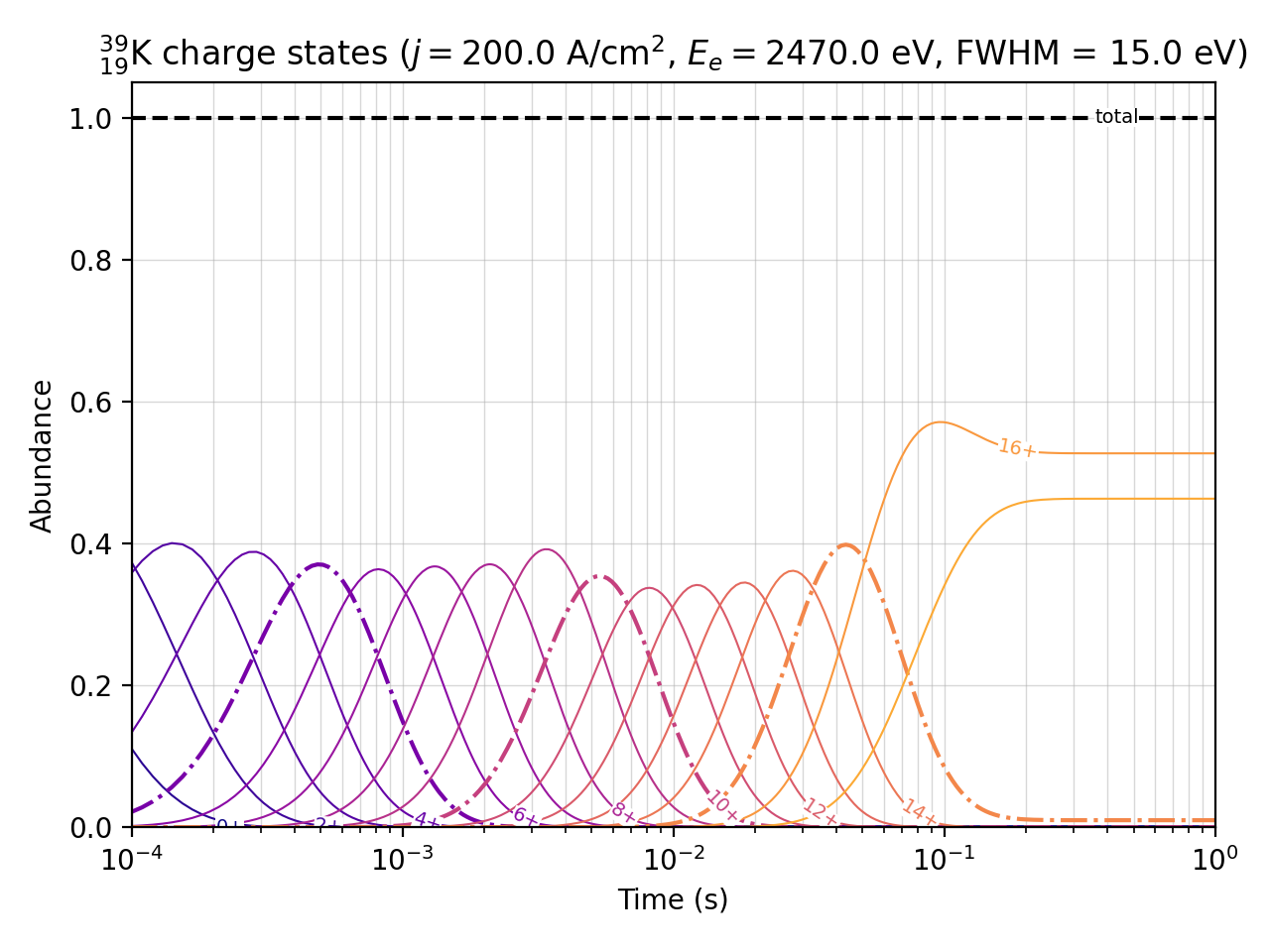
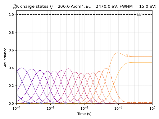
Ebisim offers a basic simulation scenario, which only takes three basic processes into account, namely Electron Ionisation (EI), Radiative Recombination (RR) and Dielectronic Recombination (DR). DR is only included on demand and depends on the availability of corresponding data describing the transitions. Tables with data for KLL type transitions are included in the python package.

Setting up such a simulation and looking at its results is straightforward.

"""Example: Basic simulation with DR"""

from matplotlib.pyplot import show
import ebisim as eb

# For the basic simulation only a small number of parameters needs to be provided

element = eb.get_element("Potassium")  # element that is to be charge bred
j = 200  # current density in A/cm^2
e_kin = 2470  # electron beam energy in eV
t_max = 1  # length of simulation in s
dr_fwhm = 15  # effective energy spread, widening the DR resonances in eV, optional

result = eb.basic_simulation(
    element=element,
    j=j,
    e_kin=e_kin,
    t_max=t_max,
    dr_fwhm=dr_fwhm,
)

# The result object holds the relevant data which could be inspected manually
# It also offers convenience methods to plot the charge state evolution

result.plot_charge_states()

show()

(Source code, png, hires.png, pdf)

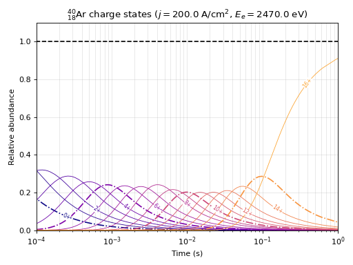
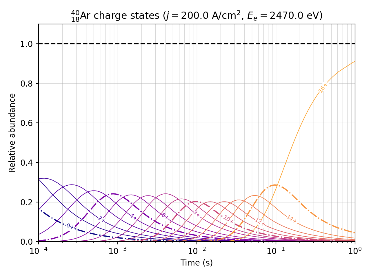
The simulation above assumes that all ions start in charge state 1+. One can easily simulate the continuous injection of a neutral gas by activating the flag for Continuous Neutral Injection (CNI).

"""Example: Basic simulation with CNI"""

from matplotlib.pyplot import show
import ebisim as eb

element = eb.get_element("Argon")  # element that is to be charge bred
j = 200  # current density in A/cm^2
e_kin = 2470  # electron beam energy in eV
t_max = 1  # length of simulation in s

result = eb.basic_simulation(
    element=element,
    j=j,
    e_kin=e_kin,
    t_max=t_max,
    CNI=True  # activate CNI
)

# Since the number of ions is constantly increasing with CNI,
# it is helpful to only plot the relative distribution at each time step
# This is easily achieved by setting the corresponding flag
result.plot_charge_states(relative=True)

show()

(Source code, png, hires.png, pdf)