Energy scans
Occasionally it may be interesting to see, what kind of impact the electron beam energy has on the charge state distribution emerging after a given time. For this purpose, ebisim offers an energy scan feature.
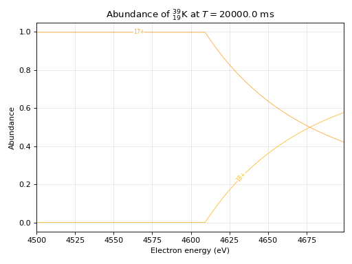
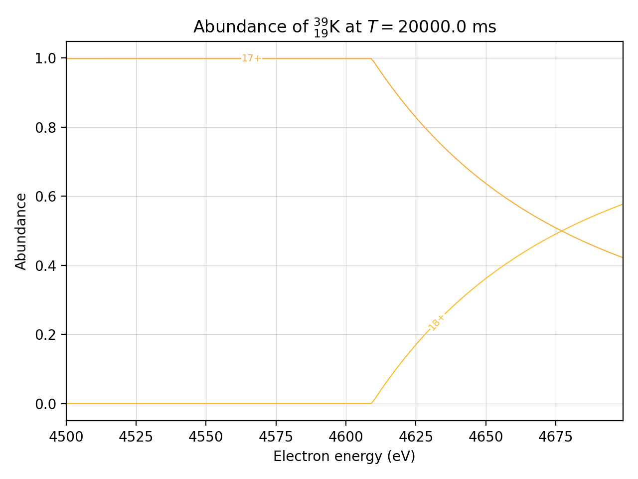
An interesting example may for example be to scan across the ionisation threshold of a certain charge state, e.g. the ionisation of potassium 17+ to 18+ opens up at approximately 4.6 keV.
"""Example: Energy scan accross ionisation threshold"""
from matplotlib.pyplot import show
import numpy as np
import ebisim as eb
# For energy scans we have to create a python dictionary with the simulation parameters
# excluding the electron beam energy.
# The dictionary keys have to correspond to the argument and keyword argument names of the
# simulation function that one wants to use, these names can be found in the API Reference
sim_kwargs = dict(
element=eb.get_element("Potassium"), # element that is to be charge bred
j=200, # current density in A/cm^2
t_max=100 # length of simulation in s
)
scan = eb.energy_scan(
sim_func=eb.basic_simulation, # the function handle of the simulation has to be provided
sim_kwargs=sim_kwargs, # Here the general parameters are injected
energies=np.arange(4500, 4700), # The sampling energies
parallel=True # Speed up by running simulations in parallel
)
# The scan result object holds the relevant data which could be inspected manually
# It also offers convenience methods for plotting
# One thing that can be done is to plot the abundance of certain charge states
# at a given time, dependent on the energies
# In order not to plot all the different charge states we can supply a filter list
scan.plot_abundance_at_time(t=20, cs=[17, 18])
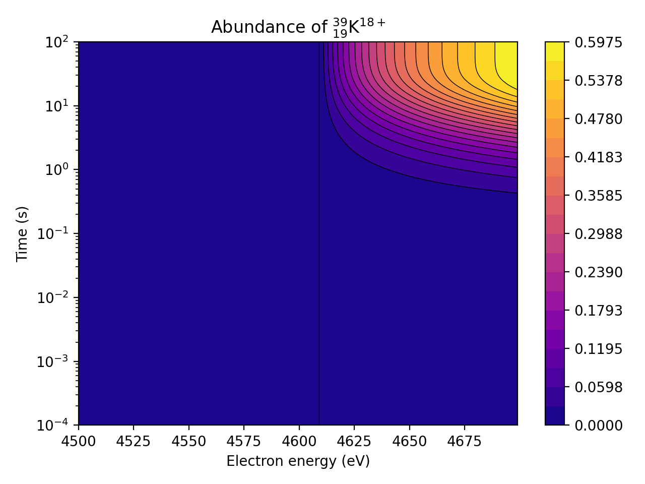
# Alternatively, one can create a plot to see how a given charge states depends on the breeding time
# and the electron beam energy
scan.plot_abundance_of_cs(cs=18)
show()

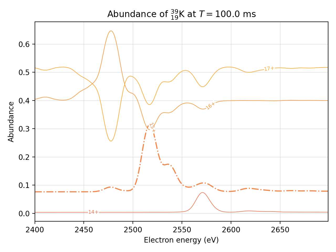
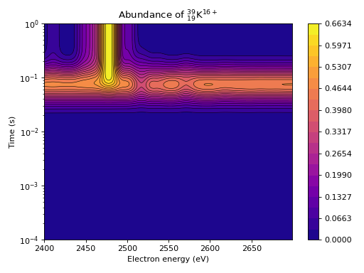
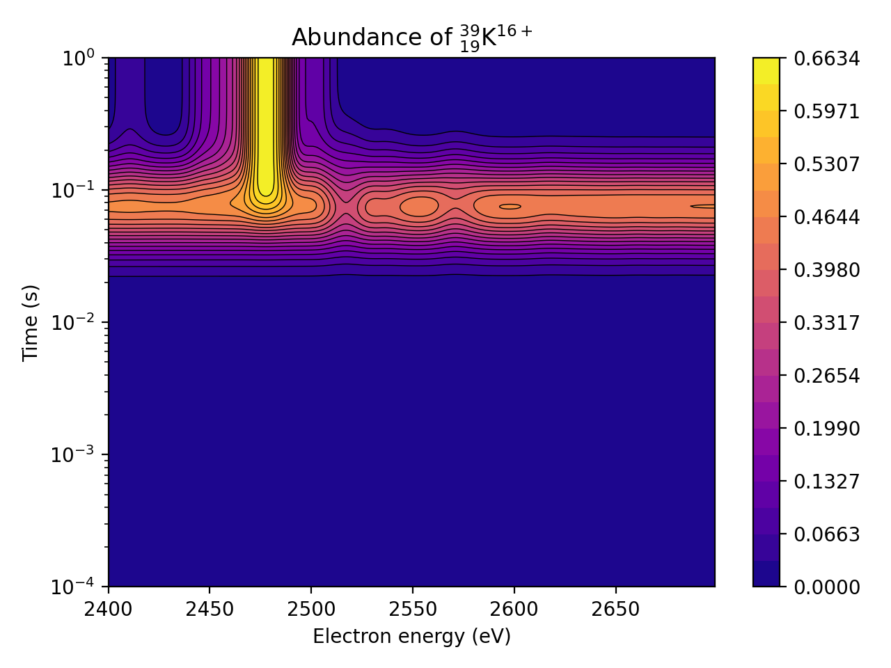
Another example, which provides structure that is a bit more interesting, is the sweep over the KLL-type dielectronic recombination resonances of potassium.
"""Example: Energy scan accross DR resonances"""

from matplotlib.pyplot import show
import numpy as np
import ebisim as eb

sim_kwargs = dict(
    element=eb.get_element("Potassium"),  # element that is to be charge bred
    j=200,  # current density in A/cm^2
    t_max=1,  # length of simulation in s
    dr_fwhm=15  # This time DR has to be activated by setting an effective line width
)
scan = eb.energy_scan(
    sim_func=eb.basic_simulation,
    sim_kwargs=sim_kwargs,
    energies=np.arange(2400, 2700),  # The sampling energies cover the KLL band
    parallel=True
)

scan.plot_abundance_at_time(t=0.1, cs=[14, 15, 16, 17])
scan.plot_abundance_of_cs(cs=16)

show()

